Contrail Regions 101 (Part I)

The thickness of persistent contrail regions

Navigational contrail avoidance is built on the premise that persistent contrail regions are (relatively) easy to avoid. These regions are generally pancake-shaped, thin vertically and broad horizontally. This post is the first in a series where we break down the structure of persistent contrail regions and how these shapes inform navigational avoidance strategies. This first post looks at the thickness of contrail regions. Stay tuned for more!

Condensation trails ("contrails") are the wispy white clouds formed behind aircraft in cold, humid patches of airspace. These man-made clouds are generally harmless, but in particularly cold and humid regions of the atmosphere they can persist and grow for hours into significant cirrus cloud formations (cirrus homogenitus).

On average, the web of contrails from the 25,000 aircraft flying around the globe produces roughly the same amount of warming as all the CO₂ emitted by aviation since 1940 (Lee et al. 2021, see our previous post Comparing Contrails and CO₂).

The good news is that it may be simple to reduce contrail warming. We can often fly around these icy regions that form persistent, harmful contrails. Re-routing flights like this is often called navigational contrail avoidance.

Navigational avoidance is built on the premise that persistent contrail regions are sparse and (relatively) easy to avoid. These regions are often pancake-shaped—very thin vertically, and broad horizontally—and can be bypassed by moving aircraft slightly up, down, or occasionally around. For the new parents out there, it's the opposite of We're Going on a Bear Hunt. We can go over it, we can go under it, we can go around it, but we mustn't go through it.

For persistent contrails to form, a region of airspace must:

1. Be cold enough to cause wet, hot engine exhaust to form ice crystals on engine emissions or pre-existing atmospheric aerosols (i.e., tiny particles). The Schmidt-Appleman Criterion (SAC) predicts these conditions.^[1] Most contrails that initially form will vaporize in a few minutes (harmless).
2. Be humid enough to freeze additional water vapor onto the initial contrail. The technical term for these atmospheric regions is ice super-saturated regions (ISSRs). When contrails form in ISSRs, they can persist and grow for many hours (potentially harmful).

When an aircraft satisfies the Schmidt-Appleman Criterion in a region of atmosphere that is ice super-saturated, we call it a persistent contrail region (PCR).

Can we avoid persistent contrails by flying higher or lower?

We often hear that ice super-saturated regions and persistent contrail regions are ~1,000 feet (or a few hundred meters) thick on average.

To put that in a relevant context, aircraft fly at specific altitudes called flight levels (FL). Flight levels are spaced out every 1,000 feet (~300 m) and labelled in hundreds of feet, e.g., FL300 = 30,000 ft, FL410 = 41,000 ft, etc. In most air traffic regimes, aircraft alternate direction every flight level (typically East-West),^[2] so if an aircraft wants to fly higher or lower, it actually must move two flight levels (2,000 ft, or ~600 m) up or down.^[3]

If contrail regions are only around a thousand feet thick, then aircraft should only have to move up or down one vertical movement (two flight levels) to avoid them.

But what's the evidence for this premise? Given the magnitude of contrail impacts and the potential to reduce them, we'd expect to see a wide literature studying the thickness of contrail regions. Surprisingly, there are only a few comprehensive studies to reference (outside a few with limited geographies).^[4]

For the rest of this post, we'll look at some of the best vertical atmospheric measurements (atmospheric soundings) to gain intuition around the thickness of contrail regions and how this informs navigational avoidance strategies.

What measurements are available?

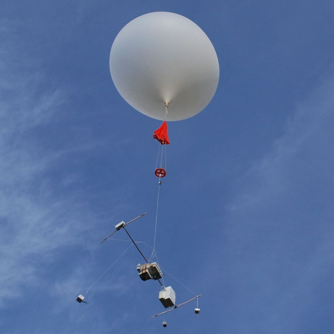
Unsurprisingly, measuring the temperature and humidity profile of a column of airspace 30,000 feet up (10,000 m) is not easy. The best data we have with any degree of coverage comes from radiosondes (or weather balloons).

Thousands of radiosondes are launched every day from all over the world, including mega-cities and remote islands. The balloons gently float up, radioing measurements of temperature, humidity and other properties back to Earth before popping high in the atmosphere, job done.

These global radiosondes would be ideal for measuring contrail region thickness, but most aren't capable of detecting thin subtle ISSRs. Luckily, we can use a subset of radiosondes known as the Global Climate Observing System Reference Upper-Air Network (GRUAN). GRUAN is an international effort providing high-quality, reference-grade measurements of the upper atmosphere from a network of stations worldwide.

GRUAN's data are renowned for their rigorous calibration, consistent methodologies, and comprehensive metadata. Crucially, GRUAN's dataset has high vertical-resolution humidity and temperature profiles, which are essential for identifying thin ISSR regions.^[5] There are lots of other radiosonde data available, but they just aren't calibrated as well as the GRUAN data, or in many cases, we don't have the raw vertical resolution to detect ISSR thickness.

We use GRUAN data in this post to explore contrail region thickness. The data spans the last decade, over 24 stations on 7 continents, with over 100,000 radiosonde launches:

See Methodology Notes for more details on how the data was processed.

So how thick are contrail regions according to the measurements?

We can look at the thickness distribution of ice super-saturated regions (ISSRs) and persistent contrail regions (PCR = SAC & ISSR) in the GRUAN data. According to the radiosondes, more than 80% of ISSRs and PCRs are less than 2,000 feet thick (2 flight levels) and about two-thirds are less than 1,000 feet thick. A very small minority—about 5%—are more than 4,000 feet thick:

Persistent contrail regions are less frequent than ISSRs but tend to be thicker than ISSRs—a conclusion also found in other radiosonde studies.^[4:1] PCRs are less frequent because they are a subset of ISSRs, and they tend to be thicker because many of the thinnest ISSRs are less likely to form contrails (i.e., satisfy SAC).

In general, PCR thickness doesn't vary much with season, time of day, and geography. Winter produces the thickest persistent contrail regions (due to lower temperatures), but the variation across season is negligible for most of the distribution. There is a modest difference in the thickest regions: ~17% of persistent contrail regions are thicker than 2,000 feet in the winter, but this falls to ~14% in the summer. Similar variation occurs between (slightly) thicker contrail regions in polar latitudes (between 60° and 90°) and thinner regions in tropical latitudes (between 0° and 30°).

How does this inform navigational contrail avoidance?

The actual thicknesses of contrail regions might not be the critical question for navigational avoidance. We'd like to know how far we have to move aircraft to find contrail-free airspace. In particular:

• How often do we encounter a PCR at a given flight level?
• Can we avoid the PCR at this flight level by adjusting up or down one vertical step (2,000 feet, or 2 flight levels)?
• How often do we need to move 4,000 feet or more?

The chart below shows the likelihood of running into a PCR (based on GRUAN data) at typical commercial aircraft cruising altitudes (FL250—FL400). The chart also shows the likelihood of avoiding the PCR with 1, 2, or 3 vertical steps (2, 4, or 6 flight levels) for an aircraft flying at a specific flight level.

Remember this analysis is only looking at PCR avoidance in one vertical column of space. In practice, avoidance might be more complicated. There might be another PCR at a different altitude slightly downstream, or we might not be able to move up or down due to traffic. We also might be at the current ceiling of the aircraft for it's payload. All these considerations have to be taken into account by trajectory and traffic optimizers. Luckily we don't have to limit ourselves to single vertical maneuvers to avoid PCRs.

The likelihood of running into a PCR on any flight level varies from about 5% to 10%, with the highest probability in FL320 and FL330. In reality, the flight level with the highest PCR probability varies a little with season and latitude, and so the peak shown here is more a reflection of the time and locations of the GRUAN dataset.

In about 30% of PCRs, one step (2,000 feet) in either direction could avoid the region (the dark grey bar). In around half of PCRs, the region could be avoided by one step up or down (2,000 feet), but not both (the dark blue bar).

So 80% of the time, a flight level change of 2,000 feet (the minimum allowed in most air traffic control systems) avoids the contrail region. Of the remaining 20% of PCRs, over 80% could be avoided by a flight level change of 4,000 feet (2 steps).

The probability that an aircraft requires three vertical steps (6,000+ feet) to avoid a PCR is less than 5% (the orange bar), typically around 3% in the most common cruise altitudes for commercial aircraft.

Conclusion

The radiosonde data clearly supports the claim that persistent contrail regions (and ice super-saturated regions) are around 1,000 feet thick. Over 80% of the PCRs and ISSRs in the GRUAN data were less than 2,000 feet. Only 5% of regions exceed 4,000 feet thick.

The data also suggests that a single vertical step (2,000 feet, or 2 flight levels) is often sufficient to move a flight out of a persistent contrail region. While this may be hard to achieve in practice, it provides empirical support for intuition built on numerical weather prediction models.^[6]

In the rest of this series, we'll look at other characteristics of contrail regions (e.g., vertical spacing of regions, breadth, frequency) and how they affect the potential for navigational avoidance.

Methodology Notes

For those interested in reproducing these results:

• Dataset includes all GRAUN data up to July 2025 from all four instruments available (Vaisala RS41 & RS92, and Meisei iMS-100 & RS-11G radiosondes).
• Pressure levels converted to geopotential height (flight levels) using International Standard Atmosphere. Radiosonde data filtered for valid temperature and humidity readings between 25,000 and 45,000 feet.
• pycontrails used to convert humidity readings to RH_ice and determine SAC using an engine efficiency of 30%.
• Persistent contrail regions were defined as where SAC is satisfied and RH_ice > 100%.
• We used a continuous region tolerance of 100 feet when defining vertical regions. This means if the data drops below the PCR threshold for less than 100 feet, the algorithm still considers it a continuous contrail region. In other words, at least 100 feet of clear air was required to define the edge of a contrail region. This has a tendency to slightly amalgamate contrail regions, but smooths sensor noise on and relative humidity measurements bouncing around 100%.
• Seasons were defined purely by date of launch and the sign of the latitude:
  • March/April/May (Spring in Northern Hemisphere, Autumn in Southern)
  • June/July/August (Northern Summer; Southern Winter)
  • September/October/November (Northern Autumn; Southern Spring)
  • December/January/February (Northern Winter; Southern Summer).

Glossary

• FL: Flight Level
• ISSR: Ice super-saturated region
• PCR: Persistent contrail region
• SAC: Schmidt-Appleman criteria

Footnotes