
Introducing ContrailBench: Measuring contrail forecasts against reality
This post describes a new framework to evaluate contrail forecasts against real-world observations.
At the recent IATA-RAeS Contrails Workshop (11–12 March 2026), we introduced ContrailBench — a framework to answer the surprisingly hard question: how good are contrail forecasts? (video here) This post introduces why we need this framework, how we're approaching it, and the methodology behind the first release.
Accurate contrail forecasts are the foundation of navigational contrail avoidance — they inform where planes should fly to reduce the climate impact of persistent contrails. Yet despite their importance, there's no agreed standard for what makes a contrail forecast "good", nor any common methodology for measuring it. There's a clear need for an objective, quantitative method to evaluate forecasts against real-world observations.
We're not the first to try to measure contrail forecast accuracy. Many studies have examined point-by-point accuracy of numerical weather predictions with in-situ sensors or satellite imagery.[1] In our previous post exploring contrail observations, we saw that observations are also imperfect, varying substantially in recall, confidence, and coverage. We want a benchmark that combines multiple observation sources to build a robust picture of forecast accuracy.
We also want a benchmark that reflects the operational realities of navigational contrail avoidance. We could forecast broad avoidance regions and capture most contrails, but routing around those regions would be operationally disruptive and costly. At the same time, forecasts don't need to be perfect to be highly effective. Small spatial errors (particularly in the horizontal direction) don't critically affect mitigation potential.[2]
With all these considerations in mind, we developed ContrailBench — a scalable forecast evaluation framework designed to work across a wide range of observation sources. Our goal is to deliver understandable, operationally relevant metrics that show the performance and tradeoffs of different contrail forecasts. The rest of this post walks through the rationale and methodology behind this first release.
This is a long technical post explaining the methods behind ContrailBench. If you want to skip right to benchmarks, the dashboard is featured at the bottom of this post, and the full report is hosted at bench.contrails.org. We'll be adding new forecasts and observation sources on a quarterly basis.
Terminology
When evaluating a prediction with a measurement, scientists often present the results with a contingency table (or a confusion matrix if you're into machine learning). These tables use terms like True Positives, False Positives, True Negatives, and False Negatives aggregated into metrics like Sensitivity, Precision, or Equitable Threat Score. The terminology can get confusing, so we'll review these metrics visually to make sure our language is clear.
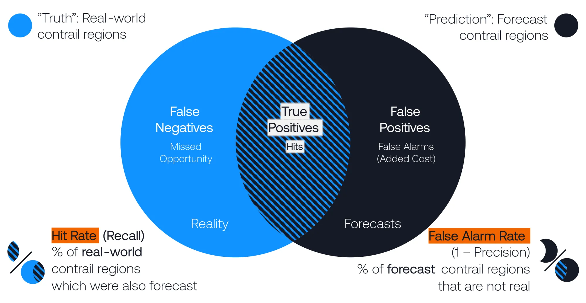
In the diagram above, the blue circle represents all true real-world persistent contrail regions (PCRs) and the black circle represents all forecasts of PCRs. Ideally, we'd like the black circle of forecasts to entirely overlap with the blue circle of true PCRs (the hatched blue-black region).
We call points in the overlap region true positives or hits. These are what we want: we forecast a contrail region, and a contrail region existed in reality.
We call points only in the blue region (inside true PCRs, but outside forecast PCRs) false negatives or missed opportunities. These are real-world contrail regions that we failed to predict, and hence missed the opportunity to avoid.
We call points in only the black region (forecast PCRs, but outside true PCRs) false alarms. These are regions we may have taken action to avoid, but without actually avoiding a contrail.
When considering the accuracy of a contrail forecast (or detection) system, there are two primary inter-dependent metrics that we are interested in:
- Hit rate is the proportion of true contrail regions that are also forecast.[3]
- False alarm rate is the proportion of forecast contrail regions that are outside of true contrail regions.[4]
There are metrics that combine hit rate (recall) and false alarm rate (precision) into a single metric, such as the Equitable Threat Score (ETS). This is widely used in evaluation of meteorological forecasts, but for reasons we'll discuss below isn't quite appropriate to use for contrail forecast evaluation (due to difficulty in proving false positives).
Observations
Before we can benchmark forecasts, we need to understand what observations we're benchmarking against. In our previous post, we categorised contrail observations into five families:
- Humidity measurements (point measurements)
- Cameras (visible/IR imagery)
- Radar systems (LiDAR and Cloud Profiling Radar)
- Heat detectors (broadband radiometers)
- Reanalysis data (data assimilation into weather models)
In ContrailBench v1, we're only testing the ability of forecasts to predict PCRs.[5] For the purpose of testing PCR forecasts, only two of our five observation families are useful: (1) humidity measurements (on-aircraft sensors and radiosondes) and (2) linear contrail detections (from ground and satellite imagers).
As discussed elsewhere, Radar, LiDAR, and radiometer measurements are very useful for other aspects of contrail science, but are less useful for purely detecting persistent contrail regions.
Reanalysis data can be used to estimate where persistent contrail regions formed, but we've left it out of ContrailBench as an observation ground-truth. These "hindcasts" are really a combination of real (but sparse) observations and a weather model. As such, they are neither independent of the observations we use, nor "true" observations themselves. Forecasts often share physics and data assimilation systems with reanalysis products, so forecasts aren't independent of reanalysis data either.
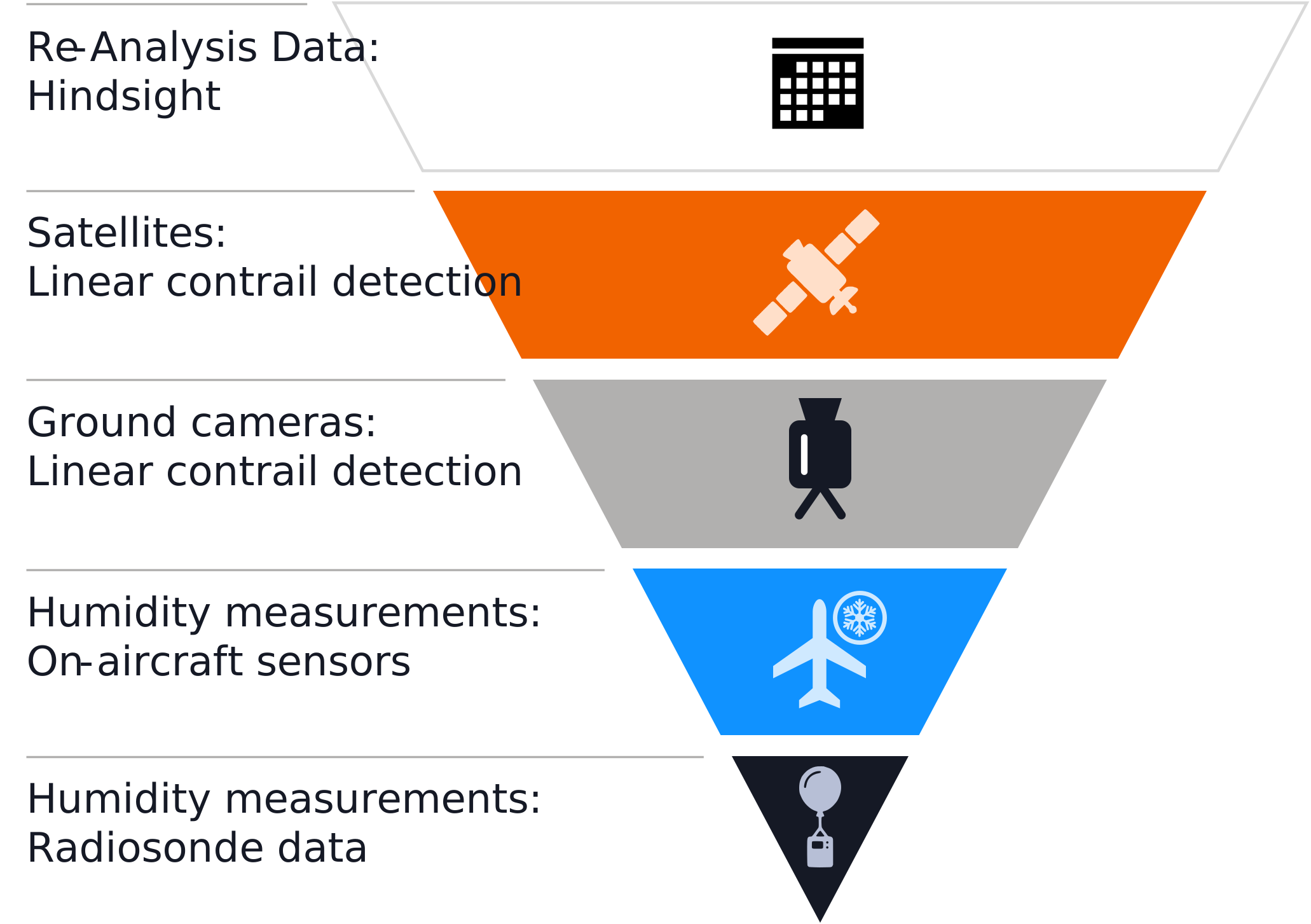
Every source of PCR observations has its own strengths and weaknesses, but all PCR observations are subject to the same nuance:
A positive PCR observation is strong evidence a PCR existed at the location. But a negative PCR observation is not strong evidence that a PCR was absent.
In the latter case, the absence of detection may be because:
- the path of a radiosonde or on-board aircraft sensor barely missed a region where persistent contrails could form
- a cloud camouflaged or obscured the view of a contrail by a satellite or ground camera
- a contrail failed to grow large enough to be detected by a camera or satellite at the time it was in view[6]
- a contrail grew into a shape that a detection algorithm doesn't recognise as a linear contrail
- a flight attribution algorithm failed to correctly match a detected contrail to the aircraft that formed it due to wind speed uncertainty or air traffic density
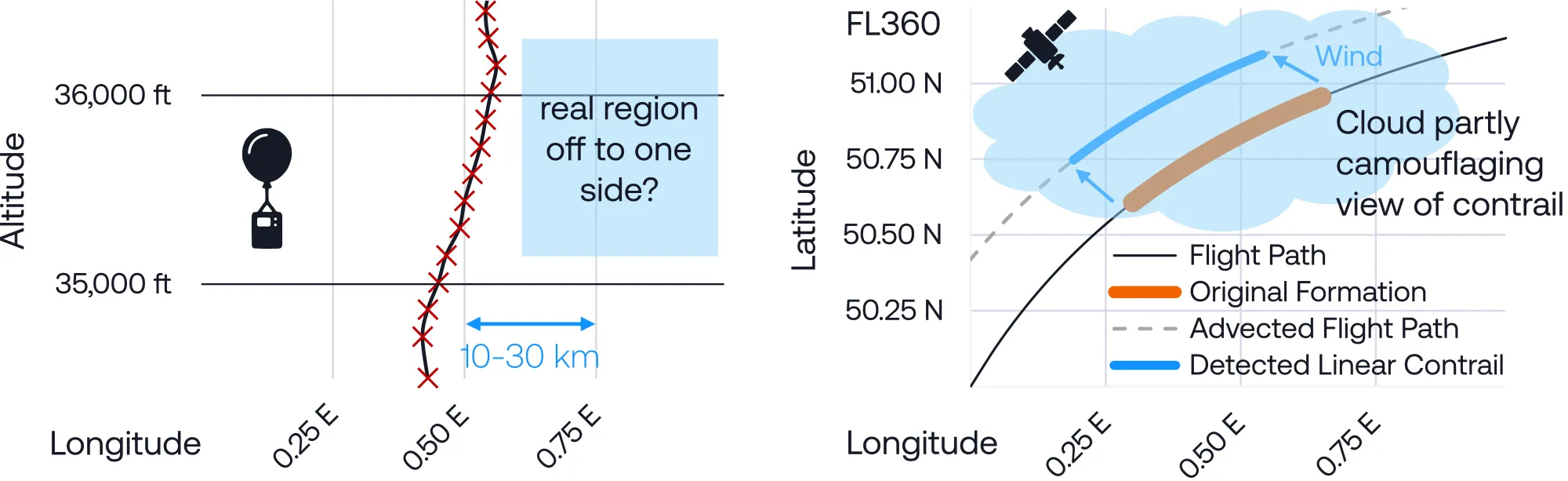
When it comes to detecting persistent contrail regions, absence of evidence is not evidence of absence.[7]
This brings us to a core challenge: PCR observations do not allow us to measure false alarms reliably. Observations allow us to confidently identify hits (true positives) and missed opportunities (false negatives). But they are poor at confirming false positives. If a forecast contrail is not observed, we cannot tell whether the forecast was wrong, or the observation simply missed it.
A shift in thinking
Rather than trying to measure false alarms directly, ContrailBench aims to reframe the problem:
We don't actually care about false alarms themselves — we care about what they cost.
False alarms only matter because they trigger unnecessary avoidance, which could add fuel burn (CO2 emissions) and other operational costs. So instead of asking "how many forecast contrail regions are wrong?" we ask "what is the cost of following this forecast?"[8]
Calculating the real cost of following a forecast is complex and depends on the systems or rules by which you conduct contrail avoidance. In ContrailBench v1, we introduce a simple proxy for the cost of avoidance: the fraction of global flight distance that lies within forecast contrail regions.[9]
Aircraft-based observations give us a sense of what this rate "should" be if forecasts were perfect. Accurate humidity measurements from IAGOS suggest persistent contrail regions cover roughly 7–9% of cruise flight distance.
If the fraction of flight distance within forecast regions is higher than the IAGOS rate, the forecast is likely overestimating contrail coverage. It's likely such a forecast will have a higher hit rate (as it's predicting more contrail regions overall), but at the penalty of a significantly increased cost. We want the forecast with the highest hit rate, with the lowest possible cost.
ContrailBench v1
The following section walks through the ContrailBench v1 methodology.
Step 1 — Build a global forecast grid
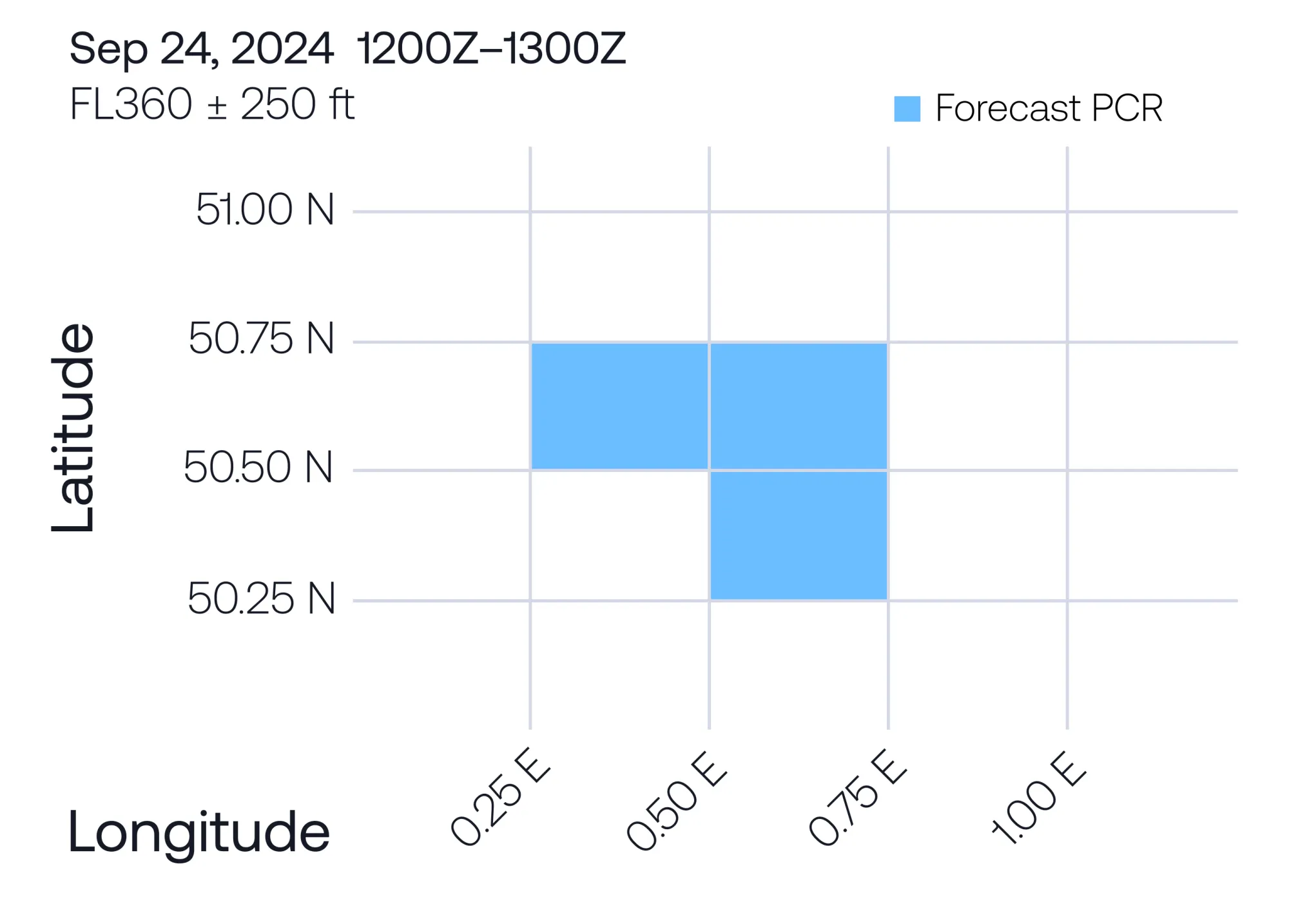
First we construct a global grid of cells:
- 0.25° longitude × 0.25° latitude [10]
- Flight levels FL270 to FL440, inclusive
- Every hour
- Across a full season or year (2024 for ContrailBench v1)
This results in ~150 billion grid cells.[11] The cells are around 28 km wide North-South, which takes a commercial aircraft around 2 minutes to cross. East-to-West they are ~28 km wide at the equator, reducing to ~14 km at ±60° latitude.
Whilst forecasts are provided at the 1,000 ft flight level intervals, we apply a ±250 ft tolerance around each flight level (effectively a 500 ft vertical band) to account for aircraft drift and measurement inaccuracies.
Step 2 — Compare forecasts to observations
In ContrailBench v1, we're evaluating forecasts against three observation datasets:
- IAGOS: A programme of accurate humidity (and temperature) sensors fitted to ~10 commercial widebody aircraft.
- GRUAN: High resolution radiosondes measuring humidity and temperature profiles from weather balloons launched from up to 30 sites 2–4 times a day.
- ContrailWatch: Google's linear contrail detections from GOES-East satellite attributed to individual flights.
These measurements provide us almost 100,000 in-situ observations of PCR cells, plus nearly 5 million PCR cells inferred from linear contrail detections, to test forecasts against:
| Observation | Total Cells | PCR Cells | % PCR |
|---|---|---|---|
| IAGOS | 804,500 | 73,087 | 9% [12] |
| GRUAN | 104,865 | 10,989 | 10% |
| ContrailWatch | 532,449,048 cells containing traffic | 4,617,000 |
IAGOS & GRUAN
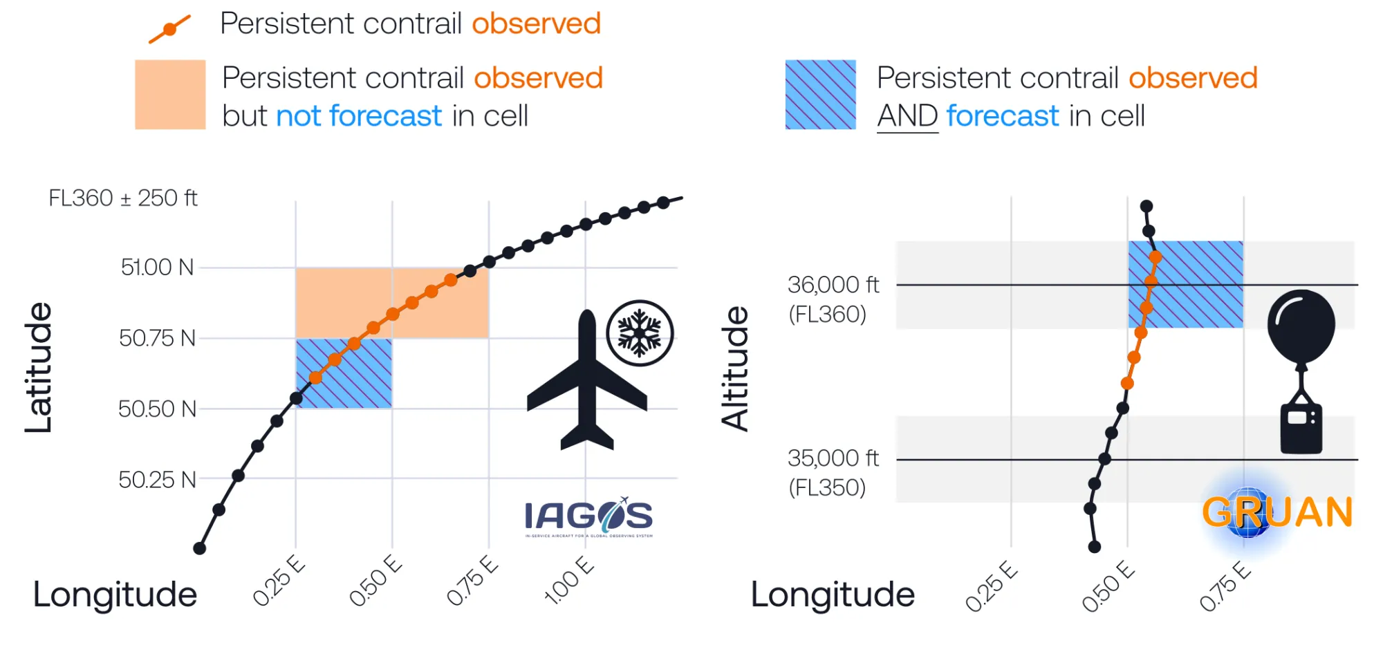
For point-measurements of humidity and temperature (IAGOS, GRUAN), we first look at all readings that fall within a given 0.25° × 0.25° cell, within the hour window, and within 250 feet vertically of the given flight level. We first remove any datapoints flagged by IAGOS or GRUAN as potential errors. Then we use humidity and temperature readings at each point to determine if the atmospheric conditions allow persistent contrail formation, i.e., if the conditions meet the Schmidt-Appelman criterion (SAC)[13] and are >100% saturated relative to ice (ISSR).
Currently, if any datapoint within the cell is PCR-positive, the cell is determined to have an observed persistent contrail region within it and is marked positive.[14] In future versions, we'd like to use all the readings in a cell to determine a probability that there is a persistent contrail region somewhere within that cell.
ContrailWatch
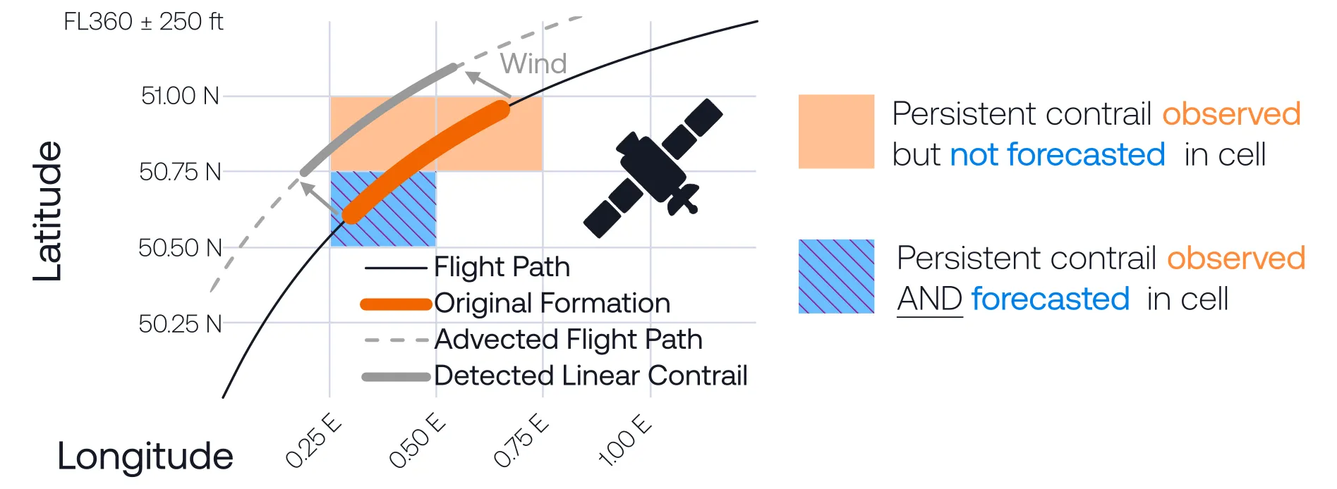
The analysis is slightly simpler with linear contrail detections. These detections are actual observed persistent contrails, not underlying humidity and temperature. We only use detections that can be attributed back a forming flight because we need to know where the contrail originally formed.
In ContrailBench v1, we're only using geostationary satellites to detect linear contrails. Geostationary satellites observe contrails ~15–30 minutes after they form, once they have reached a certain size. We assume these detections represent persistent contrails.
Similar to point measurements, if a grid cell contains just one positive observation, we count that grid cell as having an observed PCR. This is consistent with the principle discussed earlier that a lack of observed contrails is not good evidence of absence of contrails.
Analysis
For each observed contrail cell:
- If the forecast predicted a persistent contrail region, we label the cell → Hit
- If the forecast didn't predict a persistent contrail region, we label the cell → Miss
The Hit Rate is the number of Hits divided by (Hits + Misses) for each observation dataset.[15]
Step 3 — Compute operational cost
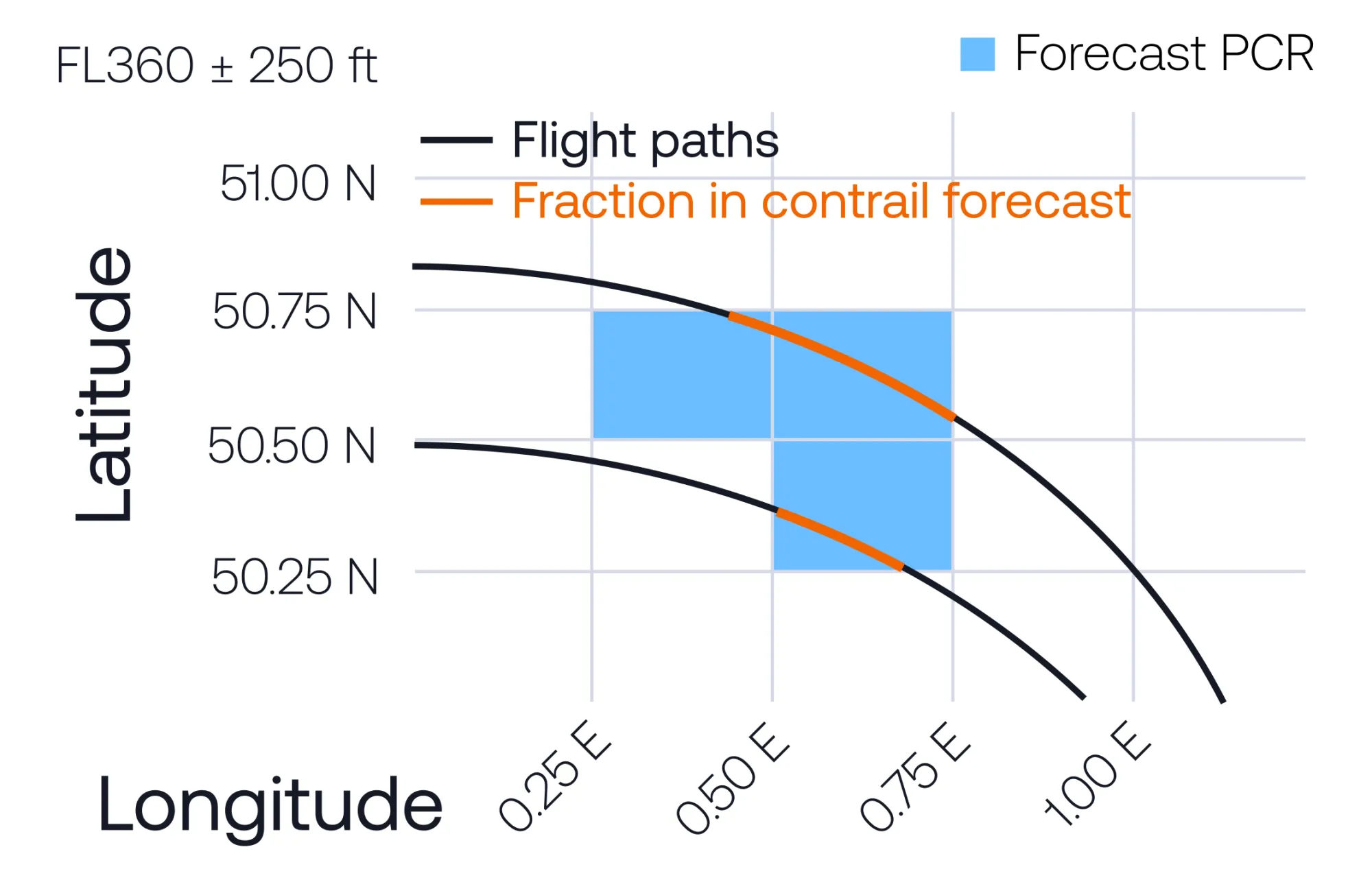
In ContrailBench v1, our cost proxy is straightforward. We simply calculate the fraction of global flight distance that falls within forecast PCR cells. We use both terrestrial and satellite ADS-B data covering all flights across the globe for a year to calculate this.
Step 4 — Build the cost–benefit curve
ContrailBench reduces forecast evaluation to a simple question: how many persistent contrails do you avoid, for how much cost?. We create a cost–benefit frontier for each forecast by varying forecast sensitivity and repeating Steps 1–3 at each sensitivity level.
In probabilistic forecasts, each cell comes with a probability that it's a PCR or not. Varying the forecast sensitivity is straightforward: we vary the probability threshold we use to count a cell as a persistent contrail region.
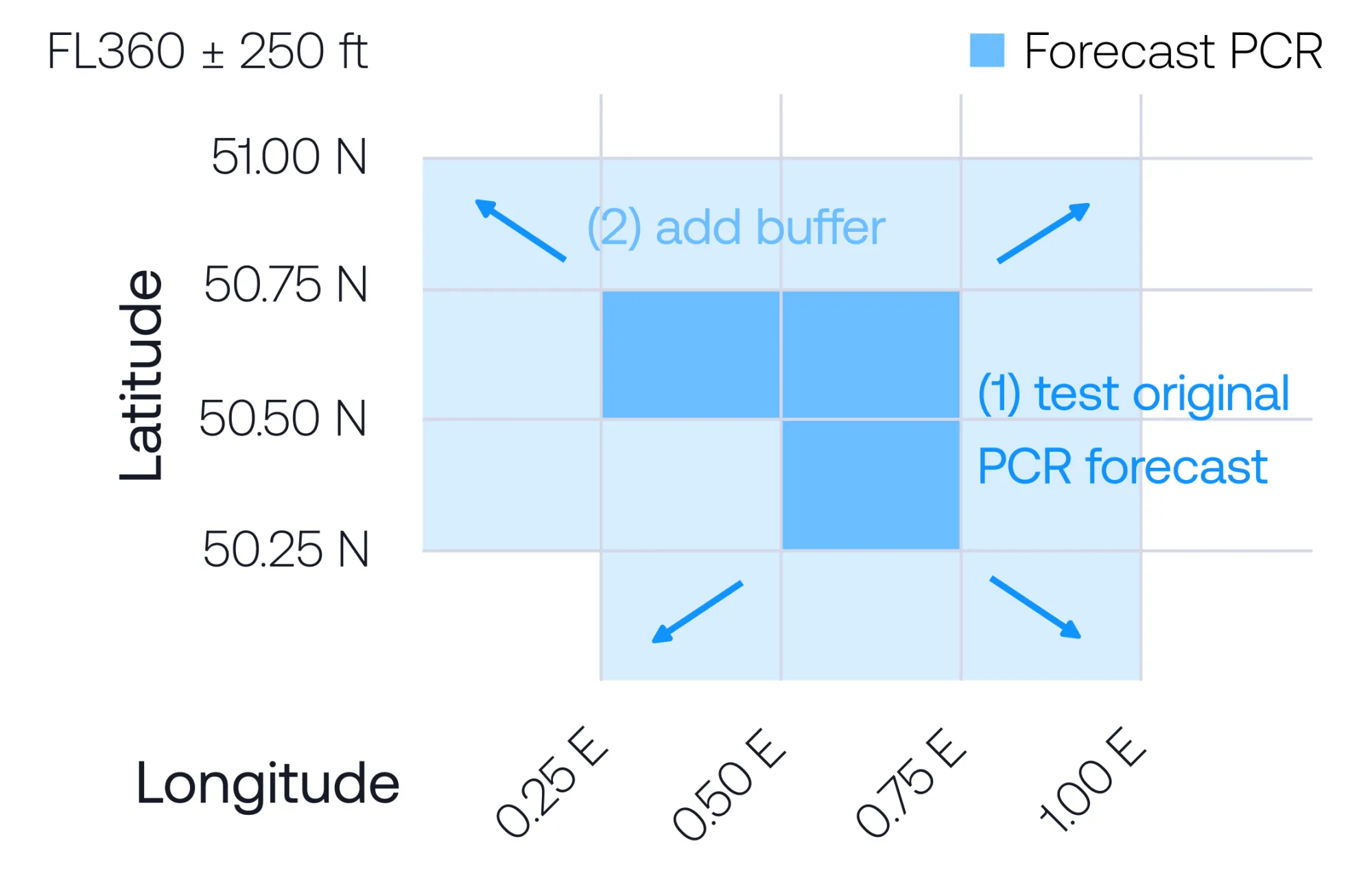
In deterministic forecasts, the forecast cells are binary; i.e., this cell is a PCR, this one isn't. In this case, we start with the deterministic forecast, and then dilate the horizontal area of each region by one 0.25° × 0.25° grid cell in every direction (horizontally) in effect expanding the total forecast areas.[16] We then repeat consecutively, adding another grid cell in each direction each time.
Example Output
Let's look at an example applying the ContrailBench v1 framework to our own (deterministic) Contrails.org forecast:
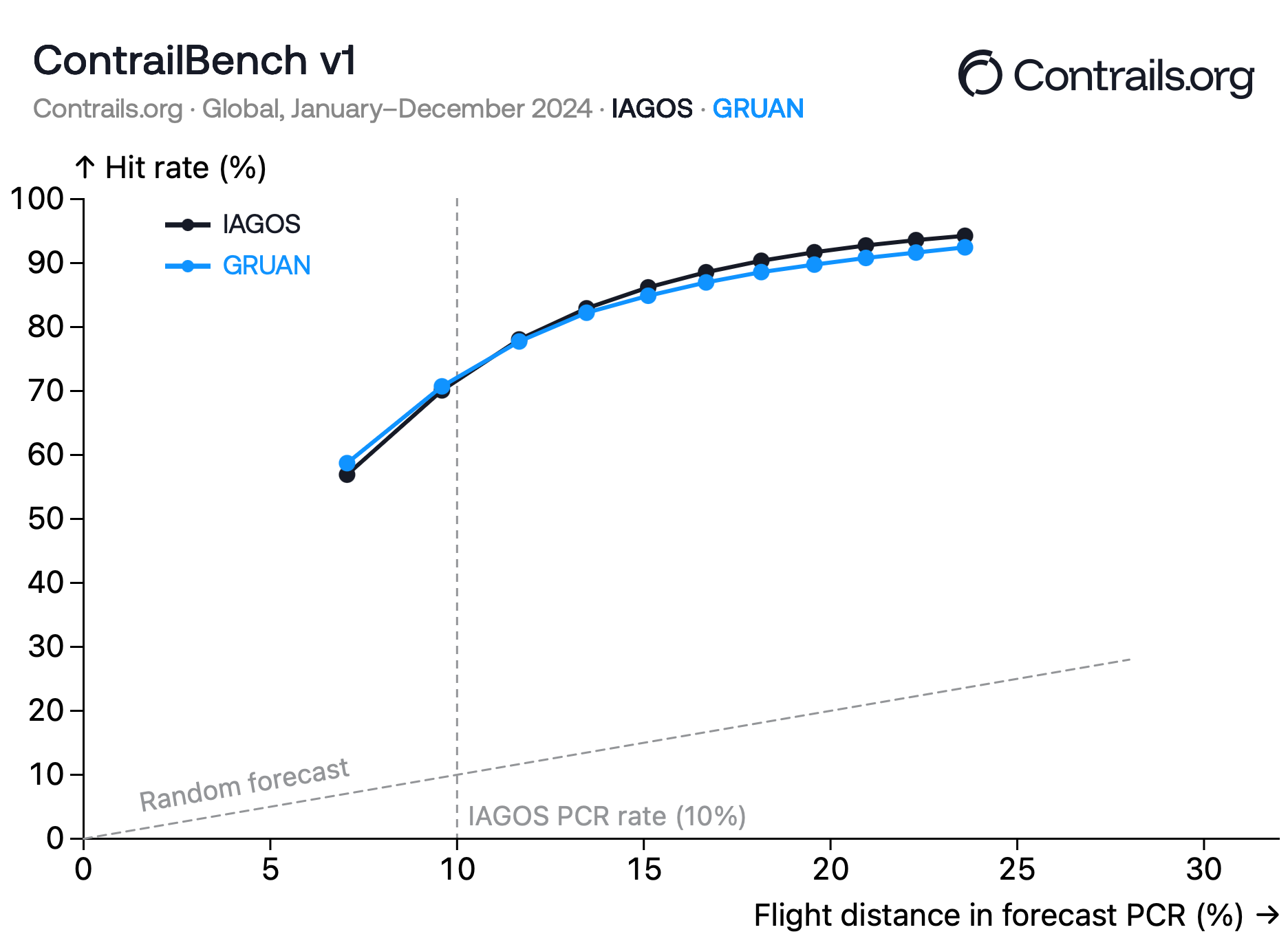
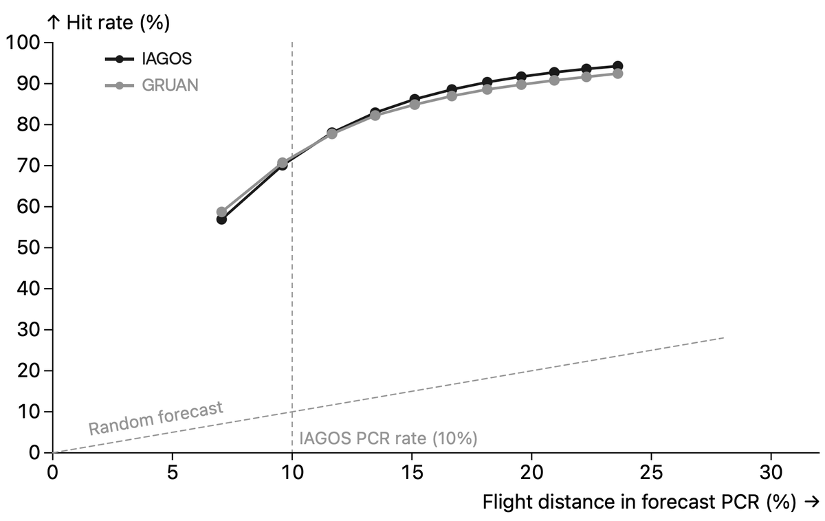
As shown in the chart, the raw forecast (before increasing sensitivity by dilating) has a hit rate of ~60% when assessed against highly calibrated radiosondes (GRUAN) or on-aircraft sensors (IAGOS).
Hit rates of ~50% are sometimes misinterpreted as being similar to random chance ("fifty-fifty"). This is not the case. The odds of correctly "guessing" that a grid cell contains a persistent contrail region are low (about 7–9% according to IAGOS).
A PCR forecast with a hit rate of 50% is similar to saying that you have a trick to pull an Ace from a shuffled deck 50% of the time: much better than the ~8% chance you'd have based on luck! (A casino certainly wouldn't let you play with that technique).
We put a line on the chart to show how well an entirely random contrail region forecast would perform for reference. While the absolute numbers may appear modest, PCR forecasts perform about an order of magnitude better than chance.
As we add a larger horizontal buffer, the hit rate improves, exceeding 70% once forecast areas are large enough to match the fraction of global flight distance IAGOS observes as PCRs. Adding one to two grid cells (~0.25° each) around forecast regions appears to be beneficial, clearly increasing the hit rate much faster than random chance (i.e., the slope is much steeper than the random forecast line).
Unlike IAGOS and GRUAN measurements, which are global (albeit sparse), the GOES linear contrail detections used in ContrailBench v1 are limited to the continental United Status (CONUS) only. Accordingly, we omit them from global benchmarks like the chart shown above and include them in regional CONUS benchmarks available on bench.contrails.org. We find slightly lower hit rates of ~45% when assessing undilated Contrails.org forecasts using GOES linear contrail detections.[17]
Limitations and next steps
We know there are improvements we can make to ContrailBench. But rather than making the perfect the enemy of the good, we're planning on releasing a ContrailBench report quarterly, giving users updates as we make improvements to the methodology and datasets.
We've already thought about some improvements we'd like to make:
Near-term
- Add more observation datasets.
- Add more forecasts.
- Incorporate uncertainty into observations, which would allow us to layer metrics from each observation into a single set of scores, rather than presenting scores for each observation type separately.
- Improve the cost metric. It's likely that our current metric (proportion of global distance spent in forecast regions) over-penalises forecasts.[18]
Longer-term
- Move beyond binary persistent contrail regions into indications of warming level.
- Benchmark other contrail forecast outputs against observations (e.g. lifetime, coverage).
Conclusion
ContrailBench helps close the critical build → measure → learn loop needed to give confidence into how forecasts perform in the real-world. It will also drive forecast improvements by providing a feedback loop on model development.
Our early results suggest something important: forecasts may already be better than many people think. See how current forecasts are performing in the first ContrailBench v1 Report.
If you have forecasts you'd like to see included, or observation data that could enhance ContrailBench, we would love to hear from you
Dashboard
Acknowledgements
Tristan Abbott built and ran analysis for ContrailBench, with support from Zeb Engberg and Nick Masson, based on concepts developed by Paul Hodgson & the Contrails.org team.
Many thanks to the Google Contrails project team for ContrailWatch and many fruitful discussions, and the IAGOS and GRUAN programmes for observation data.
Footnotes
There are, of course, a number of studies that evaluate contrail forecasts or contrail-relevant meteorology against observations. A few notable examples:
- Gierens, K. et al. (2020) "How Well Can Persistent Contrails Be Predicted?", Aerospace; and its recent update, Gierens, K. et al. (2024) "How well can persistent contrails be predicted? – an update", Atmospheric Chemistry and Physics.
- Comparing numerical weather prediction (NWP) models to aircraft humidity measurements (IAGOS), these studies from DLR show the inherent difficulty of accurately forecasting ISSRs due to the extreme sensitivity of relative humidity to minor fluctuations in temperature and water vapor.
- Arriolabengoa, S. et al. (2025) "Modeling and verifying ice supersaturated regions in the ARPEGE model for persistent contrail forecast", Atmospheric Chemistry and Physics.
- This recent study from Météo-France evaluates ISSR forecasts (not PCR) from the ARPEGE model against IAGOS aircraft measurements and radiosonde observations.
- Hanst, M. et al. (2025) "Predicting ice supersaturation for contrail avoidance: Ensemble forecasting using ICON", Atmospheric Chemistry and Physics.
- This study from DWD evaluates ensemble forecasts of ISSRs using radiosonde and aircraft observations, exploring forecast skill and uncertainty.
- Thompson, G. et al. (2024) "On the fidelity of high-resolution numerical weather forecasts of contrail-favorable conditions", Atmospheric Research.
- This study by SATAVIA assesses the accuracy of numerical weather prediction models (including ECMWF and WRF-based systems) in capturing contrail-favourable conditions, using radiosonde and aircraft observations.
- Geraedts, S. et al. (2024) "A scalable system to measure contrail formation on a per-flight basis", Environmental Research Communications.
- This study led by Google includes an assessment of ECMWF-based contrail forecasts against linear contrail detection in GOES over continental USA.
- Agarwal, A. et al. (2022) "Reanalysis-driven simulations may overestimate persistent contrail formation"", Environmental Research Letters, Vol 17(1).
- This MIT study compares reanalysis-derived contrail formation conditions against a large global radiosonde dataset (~800,000 profiles) and finds that reanalysis weather may significantly overestimate persistent contrail formation.
Taken together, these studies provide valuable insight into the accuracy of contrail-relevant atmospheric conditions. However, relatively little work has systematically benchmarked the performance of multiple contrail forecasts against observations in a way that reflects their operational use in navigational contrail avoidance, and no framework currently exists for systematic ongoing benchmarking of forecasts as they evolve. ↩︎
- Gierens, K. et al. (2020) "How Well Can Persistent Contrails Be Predicted?", Aerospace; and its recent update, Gierens, K. et al. (2024) "How well can persistent contrails be predicted? – an update", Atmospheric Chemistry and Physics.
We showed in Dean et al. 2025 that evaluating contrail forecasts on a point-wise basis likely substantially underestimates their effectiveness for navigational avoidance. That's because point-wise metrics have no way of distinguishing between a forecast that slightly misplaces a contrail region horizontally (not a big problem) and a forecast that misplaces a contrail region vertically or fails to predict the region entirely (bigger problem). This study only compared forecasts to reanalysis, but the insights gleaned from this work informed the design of ContrailBench. ↩︎
Hit Rate is traditionally called Recall or Sensitivity, i.e., the portion of reality a forecast actually gets right, or "recalls". There's an easy way to get 100% recall: just say there's a contrail region everywhere! You can improve the Hit Rate by making the forecast more "sensitive" to input signals (and generally forecasting more regions) but this comes at the penalty of increasing the False Alarm Rate. ↩︎
False Alarm Rate (FAR) is the complement of what's traditionally called Precision (i.e.,
FAR = 100% - Precision). There's an easy way to get 0% False Alarm Rate: don't predict any contrail regions! You can bring down the False Alarm Rate by making the forecast less "sensitive" to input signals (and generally forecasting fewer regions), but this comes at the penalty of decreasing the Hit Rate (Recall). ↩︎At this stage we're not evaluating long-term persistence, warming or other contrail properties in these regions. ↩︎
It's likely that these circumstances correlate with contrails that have lower climate impact (e.g. short lifetime, or pre-existing clouds), but the current version of ContrailBench isn't assessing these properties yet. ↩︎
This is a general limitation of observational systems: detection confidence is asymmetric between presence and absence. Observation systems themselves are subject to their own precision and recall as measured against "truth" (or an even more accurate measurement). The trade-off between the precision and recall of a detection system is typically calibrated according to the ideal outcome. For instance, pregnancy tests typically have poor recall, but very high precision (low False Alarm Rates). As such, if a pregnancy test tells you you're pregnant, it's almost certain you are, but a negative might just be because the test isn't able to detect that you're pregnant yet. Pregnancy tests could be calibrated to be more sensitive, improving the hit rate and telling more individuals that they were pregnant — but this would come at the penalty of telling a few more individuals that they were pregnant when in fact they were not. ↩︎
The concept of evaluating contrail forecasts through an operational cost-benefit lens is discussed in Chapter 4 of Meijer (2024), Satellite-based Analysis and Forecast Evaluation of Aviation Contrails (Ph.D. thesis, Massachusetts Institute of Technology). Meijer demonstrates that standard meteorological detection metrics (like simple false alarm rates) are insufficient for evaluating contrail avoidance because a successful diversion requires the forecast to be correct twice—at both the original and deviated flight levels. Meijer introduces a framework to evaluate prediction systems based on the ratio of the expected benefits of avoiding a contrail versus the expected costs of the additional fuel burn required. ↩︎
The distance in forecast regions scales with cost because more airspace inside forecast PCRs → more avoidance required → higher cost. ↩︎
Currently, the size of this grid matches the resolution of forecasts we're using in ContrailBench v1, and indeed most contrail forecasts we're aware of. However, if we were to benchmark a forecast in ContrailBench that had a higher resolution, we'd determine any 0.25° × 0.25° cell (× 500 feet of altitude) that contains a forecast persistent contrail region anywhere within it to count as a positive PCR cell. Similarly, if the resolution was lower, all 0.25° × 0.25° cells that overlap with a positive PCR cell in a low-resolution forecast would themselves be classed as positive PCR cells. ↩︎
Note we don't run forecasts for latitudes above 80 degrees, but only a very tiny proportion of global flight distance is inside these polar regions. ↩︎
Eagle-eyed readers might notice that this rate varies slightly, including within this article! The fraction of IAGOS flight distance in persistent contrail conditions depends on the period of time or region considered. ↩︎
We assess the Schmidt-Appelman criterion with an engine efficiency of 30%. ↩︎
This discrete gridding of observations tends to increase the PCR rate slightly. That's because IAGOS or GRUAN might only actually measure half a given grid cell as being PCR, but in ContrailBench, we then determine the entire grid cell to be PCR. When we then measure the fraction of flight distance that falls within PCR cells, the proportion increases slightly as we're effectively "rounding up" each cell. ↩︎
In ContrailBench v1, we weight each cell by its area, as cells nearer the Poles have significantly lower area than cells at the equator. There are arguments to be made about other weightings, e.g. weighting cells based on proportion of global flight distance contained within them. In our experimentation, the weighting method doesn't make a significant difference to the outcome. ↩︎
By dilating, we're trying to vary the sensitivity of deterministic forecasts in a simple manner. This method assumes that there are small spatial errors in the horizontal direction (e.g. due to wind advection). Increasing the horizontal buffer around a contrail region generally has a limited impact on operational avoidance, since the aviation system typically operates at a lower horizontal resolution than the 0.25° × 0.25° cells we're using in a forecast. Increasing the vertical thickness of regions, however, would likely have a large impact on the cost of avoidance. We can use other approaches to vary the sensitivity of a deterministic forecast, such as varying the cut-off for ice super-saturation (e.g. 90% rather than 100%), or buffering along the direction of the wind. We plan to look into these approaches in the future. ↩︎
There are a number of possible reasons why the hit rate is lower on GOES than in-situ humidity measurements. It may be that the false alarm rate on geostationary contrail detections is greater than in-situ humidity measurements (so more of the observations the forecast "missed" might themselves be false). Alternatively, the grid sizing might be improving the hit rate of the in-situ humidity measurements (due to "rounding up" the observed contrail regions to occupy the entire 0.25° × 0.25° cells) more than it does for GOES. This is something we're working on quantifying as we improve ContrailBench. ↩︎
Increasing the horizontal buffer around a contrail region might have a very limited impact on the actual cost of operational avoidance, since air traffic control movements, pilot decisions and flight planning tools typically operate at a lower resolution than the 0.25° × 0.25° cells. At present our penalty function treats two forecasts that cover the same fraction of global flight distance equally, whereas in reality from a cost perspective, we would prefer a forecast to be vertically thinner at the expense of wider regions horizontally. ↩︎